Running Time Analysis
and performance of basic data structures
1. Running Time Analysis
To get an idea whether your solution to a problem is fast enough, i.e., will avoid a TLE (Time Limit Exceeded) verdict, it is a good idea to perform a running time analysis. This basically boils down to estimating how many steps your program will take as a function of the input size. When performing such an analysis, we always consider the worst case, but more about that later.
 Image credit: ChatGPT
You might have heard the story about how Gauss, as a school boy,
came up with the formula $\frac{(n+1)n}{2}$ for computing
the sum of the first $n$ integers, i.e.,
the value of the sum $\sum_{i = 1}^n i$.
From the viewpoint of algorithms,
you might say he found an algorithm that
is much faster than simply evaluating the sum step by step.
Let us look at both algorithms,
the first one computing the sum with a loop,
and the second one using Gauss' formula,
and let us estimate its running time, based on the ``input size'' $n$.
Image credit: ChatGPT
You might have heard the story about how Gauss, as a school boy,
came up with the formula $\frac{(n+1)n}{2}$ for computing
the sum of the first $n$ integers, i.e.,
the value of the sum $\sum_{i = 1}^n i$.
From the viewpoint of algorithms,
you might say he found an algorithm that
is much faster than simply evaluating the sum step by step.
Let us look at both algorithms,
the first one computing the sum with a loop,
and the second one using Gauss' formula,
and let us estimate its running time, based on the ``input size'' $n$.
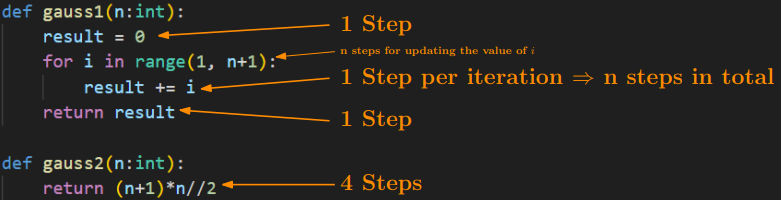
Let us consider the function
gauss1 first.
It starts by assigning the value 0 to the variable
result,
which takes one step.
Then comes the main loop which is repeated $n$ times
as $i$ goes from $1$ to $n$.
In each iteration of the loop, we increase
the value of
result
by $i$, performing one step per iteration.
This results in a total of $n \cdot 1$ steps.
Strictly speaking, we also have to count
one step every time the counter $i$ gets increased,
which gives an additional $n$ steps.
(But as we see below, we will not have to be that careful in the future.)
Lastly, the return statement in the last line of the function
also counts as one step.
In total, we have $2n + 2$ steps for executing
gauss1(n).
The function
gauss2
on the other hand takes way fewer steps:
it simply performs three arithmetic operations,
each of which count as a single step,
plus one step for the return statement.
In total, it performs only 4 steps, regardless of the value of $n$.
In summary,
as $n$ increases,
gauss1
will perform more and more steps ($2n + 2$),
and therefore become slower and slower, while
gauss2
always only takes $4$ steps, giving an answer instantly,
regardless of how big $n$ becomes.
What is a step?
Note that it is not always obvious what you can consider to be a single step.
For example, an instruction such as
x in S
may look like a single step, but the number of steps this takes
crucially depends on what kind of data structure S is.
Steps are
basic operations such as
arithmetic operations,
variable assignments,
comparisons
(==, <, <=, ...).
Note that we always assume that the values involved in these basic operations
(numbers, strings, etc) are not excessively big.
As a silly example, suppose we have two strings
x, y
that both contain
all texts that humanity has ever produced.
Then, testing
x == y
might still take a considerable amount of time.
But in general, we rarely have to take such extreme cases into account.
Big-O Notation
As algorithms get more complicated, so does their analysis. This is why we use the Big-O notation when estimating the running time of algorithms rather than meticulously counting every single step they take. For our purposes, it is enough to know that Big-O notation lets us do two things:
- Disregard constant factors.
- Remove lower-order terms in sums.
gauss1(n)
which took $2n + 2$ steps.
Using Big-O notation, we can first rewrite
$O(2n + 2) = O(2\cdot n + 2\cdot 1)$,
then use the first rule to observe that
$O(2\cdot n + 2 \cdot 1) = O(n + 1)$,
and then use the second rule which gives
$O(n + 1) = O(n)$.
This is known as a linear running time.
For
gauss2(n),
we have $O(4) = O(4 \cdot 1) = O(1)$
by rewriting and applying the first rule.
This is known as a constant running time.
Worst Case
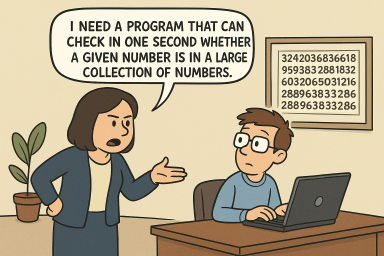 Image credit: ChatGPT
Let us consider another problem: You are given a large collection of numbers,
and you want to verify if a certain number $x$ is contained in that collection.
Your program cannot run longer than one second.
Suppose the numbers are stored in a list,
then we can simply
loop through its elements one by one, and say yes if $x$ is found,
and no otherwise:
(Observe that this is essentially what the
Image credit: ChatGPT
Let us consider another problem: You are given a large collection of numbers,
and you want to verify if a certain number $x$ is contained in that collection.
Your program cannot run longer than one second.
Suppose the numbers are stored in a list,
then we can simply
loop through its elements one by one, and say yes if $x$ is found,
and no otherwise:
(Observe that this is essentially what the
in-operator on lists does.)
def is_in(x, alist):
    for i in range(len(alist)):
        if alist[i] == x:
            return True
    return False
alist
in which case the function
is_in
will return
True
and terminate after just a few steps.
On the other hand, if $x$ is not
in the list, the function goes through all its elements before returning
False
which might take much longer.
The following graphs show empirical results of timing how long it takes to test
if the number $i$ is in the list [1, 2, ..., 200000000].
The smaller the number,
the earlier it appears in the list,
the faster the our program.
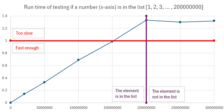
So which case should we base our analysis on? As we want a guarantee of the performance of our program, we should always focus on the worst case: This way, no matter what our input is exactly like, we always know that the program runs within the claimed bound. So for this task, our program has a running time of $O(n)$, where $n$ is the length of the list that we are inspecting. This corresponds to the worst case, when the element we are looking for is not contained in the list and we inspect every single element in the list.
Another example
Let us consider the following code, which counts how many elements of a list A are also contained in another list B.
count = 0
for x in A:
    if x in B:
        count += 1
for x in A
runs for $n$ iterations.
As discussed above, in the worst case,
the test
x in B takes $O(n)$ time,
even though it may look like a single step at first glance.
Therefore, each iteration of the loop in fact takes at most $O(n)$
steps, so the running time of the entire program is
$n \cdot O(n) = O(n^2)$,
the number of iterations times the number of steps per iteration.
The table
It is a good idea to memorize (or write down) how big inputs for an algorithm with a certain running time can get when you have a 1-second time limit. Note that these serve only as rough estimates, while the running time of your program could in principle be heavily influenced by the constants that the Big-O notation ignores, so this should be taken with a grain of salt.| $n \le \ldots$ | Running time | Comments |
| ``$\infty$'' | $O(1), O(\log n)$ | Basically anything goes. For $O(\log n)$: binary search |
| 100M | $O(n)$ | A few passes over a collection with constant-time check each. |
| 4.5M | $O(n\log n)$ | Sorting |
| 10K | $O(n^2)$ | 2 nested loops |
| 450 | $O(n^3)$ | 3 nested loops |
| [24..26] | $O(2^n)$ | Trying all subsets with constant time check per subset |
| [18..22] | $O(2^n \cdot n)$ | Trying all subsets with linear time check per subset |
| [10..11] | $O(n!)$, $O(n^6)$ | Trying all permutations, 6 nested loops |
2. Lists
We briefly discuss common methods on lists and their running times. Things you can do efficiently (i.e., in $O(1)$ time) on lists are: Retrieving or setting the value at any position $i$. Appending a new element to the end of the list, and removing the last element from the list (so-called ``popping'').
On the other hand, the following common methods may take $O(n)$ time
in the worst case.
As dicussed above, checking whether an element is contained in a list
may amount to inspecting every single element in it,
so
x in alist
may take $O(n)$ time.
Similarly, calling
alist.index(x),
which returns the lowest index $i$ such that
alist[i] == x is true,
might take $O(n)$ steps:
Again, this method loops over the elements of the list
from front to back and returns the first index satisfying
the required condition.
If the first occurrence of $x$ is at,
for instance, position $n/2$,
then we perform $O(n)$ unsuccessful checks
before finding the answer,
so in the worst case, we take $O(n)$ time.
While removing the last element can be done efficiently
using the pop-method,
removing an element from an arbitrary position may take $O(n)$ time.
Consider the case when we want to remove the element that sits roughly
in the middle of the list, say at index $n/2$.
To make sure that all elements in the second half are at the
correct position after the removal,
we have to shift each elements whose index is greater than $n/2$
by $-1$.
Since there may be about $n/2 = O(n)$ such elements,
we perform $O(n)$ operations.
The running time of
alist.remove(x),
which removes the first occurrence of $x$ in the list,
is therefore $O(n)$ in the worst case.
Calling
alist.insert(i, x)
inserts $x$ at position $i$ of the list and shifts
all elements that are currently at position $i$ and onwards
one position to the right (by +1).
Again, in the worst case we might perform $O(n)$
such shifts (depending on the value of $i$)
and therefore the running time is $O(n)$.
(Observe the difference with setting
alist[i] = x
where we simply override the value that is currently at position $i$
in the list.)
| Command | Effect | Running Time | Comments |
x in alist |
True if x is contained in alist and False otherwise. |
$O(n)$ | |
alist[i] = x |
Sets the value at position i to x. | $O(1)$ | |
x = alist[i] |
Sets x to the value at position i in the list. | $O(1)$ | |
alist.append(x) |
Attaches x to the end of the list. | $O(1)$ | |
alist.pop() |
Returns and removes the last element from the list | $O(1)$ | |
alist.remove(x) |
Removes the first occurrence of x in the list. | $O(n)$ | Raises an error if x is not in the list. |
alist.index(x) |
Returns the first index of x in the list | $O(n)$ | Raises an error if x is not in the list. [Sample problem] |
alist.insert(i, x) |
Inserts x at (before) position i in the list. | $O(n)$ |
Practice problems: list
Sorting Lists
A common task you have to perform with lists is sorting. There are two ways of sorting lists in python:
alist = [12, 2, 4, 82, 35]

sorted_list = sorted(alist) # 1st way

alist.sort() # 2nd way
alist
untouched and outputs a sorted copy of the elements in
alist.
Here,
alist
does not necessarily need to be of type list,
but any collection that python can iterate over works.
The second way modifies
alist
so that it is sorted afterwards.
Notice that this way, we lose information about the original order of the elements.
Both methods can be parameterized in certain ways:
The default way of sorting is always in
nondecreasing (increasing, smallest first) order;
if you want to sort in the opposite order, you can pass
reverse=True
as a keyword argument, e.g.,
alist.sort(reverse=True).
Another convenient keyword argument is
key,
which allows you to specify a function according to which the elements
in the list should be sorted.
For instance, the following program sorts the strings in the list
according to their length.
alist = ['hello', 'bye', 'banana', 'cart']
alist.sort(key=len)
def second_letter(x):
    return x[1]

alist = ['hello', 'bye', 'banana', 'cart']
alist.sort(key=second_letter)
lambda-functions;
the example from above can be abbreviated to:
alist.sort(key = lambda x: x[1])
A note on sorting strings in python:
Python sorts according to ASCII-betical order,
meaning that uppercase letters always come before lowercase letters.
If you want to circumvent this behavior, you can pass
key=str.lower
as a keyword argument.
Running Time. Sorting a list with $n$ elements takes $O(n\log n)$ time (assuming a single comparison can be done in constant time, which is usually the case). This means that you can sort lists with up to 4.5M elements in a 1-second time limit.
Practice problems: sorting
3. Sets
Consider the problem about testing if a number is contained in a large collection of numbers again, but assume this time the numbers are stored in a set. Then, our program is much more efficient, since testing membership in sets takes only $O(1)$ time.
This is because sets are implemented using a principle called hashing.
On a very high level, this can be explained as follows.
For the sake of argument, assume once more that your data
is stored in a data structure based on a list,
but each element, if added,
would have its designated index.
Meaning that if the element is present in our collection,
there is only one index where it can be stored.
Functions computing such indices are called
hash functions.
They take as input any element $x$, and compute its designated index
in the data structure.
When testing whether an element $x$ is contained in our data structure
it therefore suffices to compute the hash of $x$,
giving us its designated index,
and inspecting if the data currently stored at that index
is equal to $x$.
In this ideal setting, we only had to check the element at a single
position to tell if $x$ is a member or not,
rather going through all elements as we did with lists before.
Sets in python (and other programming languages) implement this principle.
There are of course certain pitfalls with this approach, most importantly
the issue of collisions.
A collision is when our hash function maps two different elements to the same index.
While in theory, this behavior can get arbitrarily bad,
in practice, we do not have to worry about it,
as there are (both time- and memory-) efficient hash functions
with great performance.
We can therefore
view the hash functions underlyings sets as
black boxes that take $O(1)$ time to compute
(again, assuming the elements we consider are not prohibilively large),
and that this enables us to do set membership testing in $O(1)$ time.
Thanks to hasing, also adding and removing elements to/from sets
can be done in $O(1)$ time.
| Command | Effect | Running Time | Comments |
x in S |
True if $x \in S$ and False otherwise. | $O(1)$ | |
S.add(x) |
Adds $x$ to $S$. | $O(1)$ | |
S.remove(x) |
Removes $x$ from $S$. | $O(1)$ | Raises an error if $x \notin S$. |
S.discard(x) |
Removes $x$ from $S$. | $O(1)$ | Does not raise an error if $x \notin S$. |
S.union(T) |
Returns $S \cup T$ | $O(n)$ | |
S.intersection(T) |
Returns $S \cap T$ | $O(n)$ | |
S.intersection_update(T) |
Sets $S$ to $S \cap T$ | $O(n)$ | |
S.difference(T) |
Returns $S \setminus T$ | $O(n)$ | |
S.difference_update(T) |
Sets $S$ to $S \setminus T$ | $O(n)$ |
Practice problems: set
4. Dictionaries
Coming soon.
Practice problems: dictionary
5. Doubly-Ended Queues (Deque)
 Image credit: ChatGPT
As we have seen above, the end of lists can be manipulated efficiently.
With
Image credit: ChatGPT
As we have seen above, the end of lists can be manipulated efficiently.
With
alist.append(x)
we can attach the element x to the list in $O(1)$ time,
and with
alist.pop(),
we can remove the last element in the list in $O(1)$ time.
In several applications, it is vital to have the same type of access to the first element of a list.
Think for instance about simulating queues:
whenever a new person arrives, they go to the end of the queue,
so we should be able to ``append'' efficiently.
And when the next person is called, they should be removed from
the front of the queue,
so we would like to be able to ``pop'' the front of the queue efficiently as well.
A deque (doubly-ended queue) is a data structure which provides that. It is an ordered data structure, just list a list, but it allows for efficiently appending and popping the front (the ``left''). To be able to use this data structure, you have to import it from the collections module. Here is how you import it and initialize and empty deque:
from collections import deque
q = deque()
| Command | Effect | Running Time |
q.append(x) |
Appends x at the end of q. | $O(1)$ |
q.appendleft(x) |
Attaches x at the front of q. | $O(1)$ |
q.pop() |
Returns and removes the last element of q. | $O(1)$ |
q.popleft() |
Returns and removes the first element of q. | $O(1)$ |
Practice problems: deque
6. Binary Min-Heaps
 A binary min-heap with list representation
If you want to know how the heap algorithms work, you can check this wikipedia entry. What makes heaps so efficient is that all its operations can be performed within a time bound that is proportional to the height of the tree representation, which is roughly $\log n$.
heapq-module
(link to python doc)
which contains an implementation of the heap algorithm
and lets you manipulate lists that store binary heaps.
You can use it as follows:
import heapq

h = []
heapq.heappush(h, 5) # Insert 5 into the heap
heapq.heappush(h, 2) # ...
heapq.heappush(h, 3)
print(h[0]) # Access the minimum element
x = heapq.heappop(h) # Retrieve and remove the minimum element
| Command | Effect | Running Time |
h = [] |
Initialize an empty list (heap) | $O(1)$ |
h[0] |
Access the minimum element in the heap h | $O(1)$ |
heapq.heapify(h) |
Turns the list h into a heap | $O(n)$ |
heapq.heappush(h, x) |
Inserts x into the heap. | $O(\log n)$ |
heapq.heappop(h) |
Returns and removes the minimum element in h | $O(\log n)$ |
By default, heaps have the minimum as a priority.
The variant that prioritizes the maximum element,
a so called max-heap,
is implemented in the heapq-module as well,
but only since python version 3.14!
Simply attach
_max
to the function names from the table above
to maintain a max-heap,
for instance
heapq.heappush_max(h, x).
You can also simulate a max-heap by a min-heap
and multiplying the priorities by $-1$.
Practice problems: heap