NHH Code

One of the most fundamental questions you can ask about a graph $G$ is: given one of its vertices $v \in V(G)$, what other vertices in $G$ can we reach from $v$ by repeatedly moving along the edges of $G$? Graph traversals are algorithms that systematically (and very efficiently!) explore the vertices of a graph, starting from a given vertex; thereby enabling us to answer the previous question and, as we see below, some other interesting questions about the structure of a graph as well. Breadth-first search (BFS) is one such graph traversal. Among its killer applications are computing shortest paths in unweighted graphs and testing whether a graph is bipartite (has no cycles of odd length).

1. How it works

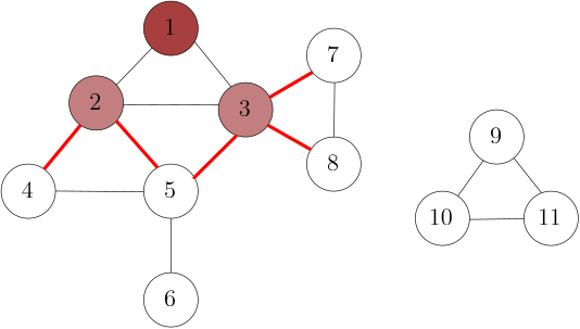Illustration of the principle of a BFS starting in vertex $1$. Click the image to start the animation. A breadth-first search of a graph $G$ starting in a vertex $v \in V(G)$ explores the graph in layers, moving further and further away from the starting vertex $v$. (If you can stomach it) you may mentalize this process like the growing of a mold starting in a fixed position and spreading in all directions at equal speed, see this youtube-video for a nice illustration (recommendation: playback speed between 0.25x and 0.5x). The initial layer $L_0$ contains only the vertex $v$ itself, the first layer $L_1$ contains the neighbors of $v$, the second layer $L_2$ contains the neighbors of the vertices in $L_1$ that have not been explored yet, i.e., that are not contained in $L_0 \cup L_1$. Generally, the $i$-th layer contains the neighbors of the $(i-1)$-th layer that have not been explored so far, meaning they are neither in layer $i-1$ nor in layer $i-2$, or any earlier layer. Formally, $L_i = N_G(L_{i-1}) \setminus (L_{i-1} \cup L_{i-2})$. Note that no pair of adjacent vertices can ever be further than one layer apart from each other, so we do not need to explicitly disregard vertices from any layer $L_j$ with $j < i-2$ in this expression.

The full Python code is as follows. We assume that the graph is provided in the neighborhood set format.

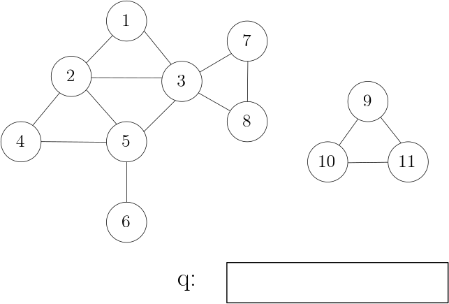Illustration of the BFS-algorithm starting in vertex $1$. Click the image to start the animation.

from collections import deque

def bfs(graph, v):
    marked = set()
    marked.add(v) # Initially, only the starting vertex v is marked.
    q = deque([v]) # The queue with vertices to visit next.
    while q: # while there are vertices left to visit
        u = q.popleft() # get and remove the vertex from the front of the queue
        for v in graph[u]: # visit u
            if v not in marked: # for each unmarked neighbor v of u
                marked.add(v) # mark v
                q.append(v) # add v to the end of the queue
    return marked
                    

Note that the above code simply returns the vertices that were marked during the BFS. Most problems require you to make modifications to the algorithm to answer the question at hand and/or to run it several times; below we see some examples. It is therefore a good idea to familiarize yourself closely with how this algorithm works.

Running time. Each vertex is marked and appended to the queue at most once (see the innermost if-statement). Therefore, each vertex is visited at most once. This in turn implies that each edge $uv \in E(G)$ is considered at most twice: once when visiting $u$ and once when visiting $v$. The remaining operations can be performed in $O(1)$ time, thanks to the efficient deque data structure. This means the overall running time is $O(|V(G)| + |E(G)|)$, or linear in the size of the graph.

2. Computing connected components

To build your intuition, take a moment and think about the following question; you may look at the graph above for an example: When a BFS starting in vertex $v$ finishes, what exactly are the vertices that have been marked?

The marked vertices are precisely those that can be reached from $v$ by moving along any number of edges, in other words, all vertices that are connected to $v$ via a path (a sequence of distinct vertices $v_1, \ldots, v_\ell$ such that $v_1 = v$ and $v_i v_{i+1} \in E(G)$ for all $i$). This set of vertices is known as the (connected) component of $G$ containing $v$. In the example above, the marked vertices after the BFS starting in $1$ are $\{1, 2, 3, 4, 5, 6, 7, 8\}$ (the connected component containing $v$), and the unmarked ones are $\{9, 10, 11\}$.

If we want to compute all connected components of a graph, we can first store a copy $U$ of $V(G)$ as the set of unmarked vertices, take any unmarked vertex $u \in U$, compute its connected component $C_u$ using the algorithm above, remove $C_u$ from $U$, and repeat until $U$ is empty. Once no vertex is unmarked, every vertex has been visited, so we have computed all connected components.

Practice problems: Where's My Internet?? Money Matters

3. Computing shortest paths...

One of the most fundamental graph problems in computer science is the Shortest Path problem, where we are given a graph $G$ with edge weights, and two vertices $s, t \in V(G)$, and we want to find a path in $G$ going from $s$ to $t$ with overall minimum weight. Think of the graph as a map; its vertices are the cities, the edges tell you between which cities you can travel and the weights say how long it takes to go from one city to another; $s$ as a city where you want to start a trip and $t$ the destination. The shortest path from $s$ to $t$ would tell you the quickest way of travelling from $s$ to $t$.

While BFS cannot handle arbitrary edge-weights, there are two interesting subcases of the Shortest Path problem that can be solved with BFS.

3.1 ...in unweighted graphs

The first case is when all edges have the same weight, say $1$. Then, a shortest path is one that minimizes the number of edges. If we start a BFS in vertex $s$, then the distance to vertex $t$ is simply its layer number (see the graph above for an example). To convince yourself of that, recall that the vertices in layer $1$ are the neighbors of $s$, the vertices in layer $2$ are the neighbors of the vertices in layer $1$ that are not adjacent to $s$, the vertices in layer $3$ are the neighbors of the vertices in layer $2$ that cannot be reached from $s$ by using at most $2$ edges, and generally, the vertices in layer $i$ are the ones you can reach from $s$ by going over $i$ edges but not by going over $i-1$ or less edges. Therefore, if the layer number of $t$ is $i$, then the distance from $s$ to $t$ is $i$.

Let us see how to modify the above code to compute the layer numbers of vertices as well. Say we want to start a BFS at vertex $v$. We use an additional dictionary and initially, we only set the layer number of $v$ to $0$. That is, we add the following line to the initialization phase of the BFS:

layer = {v : 0}
                        

for v in graph[u]: # visit u
    if v not in marked: # for each unmarked neighbor v of u
        marked.add(v) # mark v
        layer[v] = layer[u] + 1 # set the layer number of v
        q.append(v) # add v to the end of the queue
                        

Practice problems: Interplanetary Tunnels Horror List Grid

3.2 ...in 0/1-weighted graphs

The second case is when all edges have weight either 0 or 1, that is, you can use some edges ``for free'' while for the others, you pay the same amount. We can solve this problem using a slightly modified variant of BFS essentially as efficient as the standard BFS. Throughout, we assume we have a 0/1-weighted graph $G$ and we denote the starting vertex of a BFS as $s \in V(G)$.

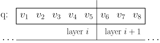State of the queue during a BFS. The crucial observation is the following. At any point during a (regular) BFS, the queue has the following shape: It consists of a prefix of vertices that are in some layer $i$, followed by a suffix of vertices in layer $i+1$. At no point we will have three or more layers with vertices in the queue. In terms of distances, the vertices in the prefix have distance $i$ from $s$ and the vertices in the suffix have distance $i+1$ from $s$. (Note that the suffix may be empty.) In the case of 0/1-edge weights, a small modification to the algorithm suffices to maintain this property of the queue. When we visit a vertex $v$ and it has a weight-$0$ edge to an unmarked vertex $w$, then we insert $w$ at the front of the queue rather than the back, as it has the same distance from $s$ as $v$. If we discover a weight-$1$ edge to an unmarked vertex $w$, we place $w$ at the end of the queue just as before.

Before we proceed with discussing the code of the 0/1-BFS, recall how to represent edge-weighted graphs. Again we will use the neighborhood set representation, as we need to iterate over neighborhoods just like above.

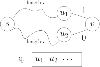A situation in 0/1-BFS where marking could go wrong. We will make one more conceptual change to the BFS which concerns how we deal with marking. The reason is the following: suppose the two next vertices in the queue are $u_1$ and $u_2$ (in that order) and they have the same distance $i$ from $s$. Both $u_1$ and $u_2$ are adjacent to another vertex, $v$, but the edge $u_1 v$ has weight $1$ and the edge $u_2 v$ has weight $0$. Applying the marking scheme of BFS ``literally'' we would mark $v$ and insert it into the queue when seeing the edge $u_1 v$ and ``set'' its distance to $i+1$. When the edge $u_2 v$ is discovered later, $v$ is already marked and therefore ignored. However, the distance of $v$ is actually $i$, observable by the length-$i$ path from $s$ to $u_2$ and then using the weight-$0$ edge $u_2 v$.

We therefore ``relax'' the marking procedure as follows. Instead of keeping a set of marked vertices, we keep the distances $d(v)$ of the starting vertex to the vertex $v$, for all $v \in V(G)$. We initially set distances of vertices except $s$ to $\infty$. Whenever we visit a vertex $u$, we go over its neighbors $v$ and if $d(u) + w(uv)$, the length of an $(s, u)$-path followed by the edge $uv$, is smaller than the value currently stored at $d(v)$, we insert $v$ into the queue in the appropriate place. Observe that this does not make the algorithm significantly slower, as any vertex will be inserted into the queue at most twice. Therefore, the overall running time remains $O(|V(G)| + |E(G)|)$.

from collections import deque
from math import inf

def zoBFS(graph, s):
    d = {v : inf for v in graph} # Set all distances to infinity.
    d[s] = 0 # The distance from s to s is 0.
    q = deque([s])
    while q:
        u = q.popleft()
        for (v, x) in graph[u]: # v is a neighbor of u and uv has weight x
            if d[v] > d[u] + x: # The current distance to v is larger than d(u) plus x
                d[v] = d[u] + x
                if x == 1: 
                    # The edge had weight 1, append v at the end of q.
                    q.append(v)
                else:
                    # The edge had weight 0, append v at the front of q.
                    q.appendleft(v) 
    return d
                    

Practice problems: Ocean Currents

4. Testing bipartiteness

Coming soon.